
AS/AD Model
Updated 6/20/2019 Jacob Reed
I would venture to say the AS/AD model of the economy is the most common element you will find on the AP Macroeconomics Exam.
This is because the AS/AD graph encapsulates the entire economy in 3 curves and illustrates the 3 macroeconomic goals of full employment, price stability, and growth. Let’s get an AP Macroeconomics Review of the different aspects of the AS/AD model. Then, don’t forget to test your knowledge with the AS/AD Graph Flash Review Game.
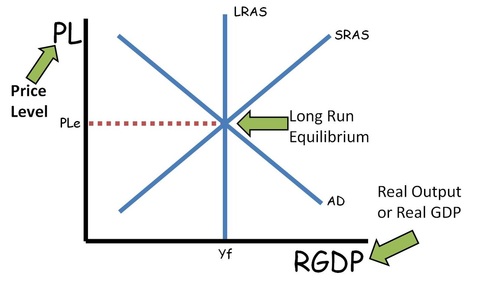
The Axes: The Y axis on the AS/AD graph is the price level (or PL) for goods and services in the economy. Think of it as the GDP Deflator or the Consumer Price Index. On the X axis, is Real GDP; which means it has been adjusted for inflation. At any point on the graph, you can multiply the price level by the Real GDP to get the Nominal GDP for that point. It is important to note that the X axis correlates to the amount of employment; more Real GDP means more employment (lower unemployment). The X axis also represents National Income (“Y”).
Aggregate Demand: The downward sloping aggregate demand curve shows the inverse relationship between the Price Level and Real GDP. This is explained by the wealth effect (assets buy fewer real goods when price levels rise), the interest rate effect (higher price levels correlate to higher nominal interest rates which correlate to less gross investment), and the net export effect (higher price levels mean fewer exports).
Aggregate demand shifters include each of the components of the output expenditure formula for GDP. Anything that would increase Consumption, Gross Investment, Government Purchases, or Net Exports will shift the AD curve to the right. A reduction in any of these will cause the AD curve to shift left. When price levels rise from a rightward shift of the aggregate demand curve, it is called “demand pull inflation.”
Many AP Macroeconomics questions have focused on government and Federal Reserve influences on the AD curve. Expansionary Fiscal policy (reducing taxes, increasing spending, or both) shifts the AD curve to the right and Contractionary Fiscal policy shifts the AD curve left (These actions also impact the Loanable Funds Market and in turn, the long-term growth rate of the economy). Federal Reserve actions in the Money Market, serve to shift the AD Curve (mostly the Gross Investment portion) through changes in the interest rate. Increases in the money supply reduce interest rates and shift AD right. Decreases in the money supply raise interest rates and shift AD left.
Short-run Aggregate Supply: The upward sloping aggregate supply curve shows a direct relationship between the Price Level and Real GDP. As prices rise, so do production levels (in the short run). This curve is upward sloping as resource prices are sticky in the short run (they do not immediately adjust to new price levels). The shifters of the SRAS curve include the prices of resources (especially wages), productivity, inflation expectations, subsidies or taxes on businesses (taxes generally move AD, but if the question asks specifically about taxes on businesses, the SRAS or LRAS may move), and Government regulations. When price levels rise from a leftward shift of the SRAS, it is called “cost push inflation,” or “stagflation” which means there is a recession and inflation at the same time.
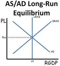
Long-run Aggregate Supply: The LRAS curve is vertical at the full employment output (“Yf”, the Real GDP that correlates to the Natural Rate of Unemployment or zero cyclical unemployment). It is vertical because, in the long run, wages and resource prices are flexible and adjust to the price level; meaning regardless of the price level the economy will produce at the full employment output. The LRAS shifts with anything that shifts the Production Possibilities Curve. So changes in the quality or quantity of resources, productivity, or technology shift the LRAS just as they shift the PPC.

Short-Run Equilibrium: This is the price level and Real GDP where SRAS and AD intersect. If the quantity (RGDP) is to the left of LRAS, the economy is experiencing a recessionary gap (it is producing less than its long-run potential). If the quantity of output is to the right of the LRAS, the economy is experiencing an inflationary gap.
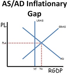
Long-Run Equilibrium: In the long run, the SRAS and AD curves will intersect at the LRAS (“Yf” – full employment output). If the economy is experiencing an inflationary gap, workers will eventually seek and get higher wages. These higher input costs shift the SRAS curve to the left bringing the economy back to full employment. If the economy is experiencing a recessionary gap, workers will eventually accept lower wages. These lower input costs shift the SRAS curve to the right bringing the economy back to full employment. Since returning to long-run equilibrium may take a very long time, fiscal and/or monetary policy can be used to get the economy back to full employment more quickly (by shifting the AD curve).
Up Next:
Review Game: AS/AD Model Review Activity
Graph Drawing Practice: AS/AD Model
Content Review Page: Loanable Funds Market Graph