What Do I Need to Know About Cost Curves?
Updated 9/1/2023 Jacob Reed
Costs
Implicit and explicit costs were already covered in the cost revenue, and profit review. Below are more costs you need to know and each of them includes both implicit and explicit costs.

The total cost curves are important, but pay special attention to the average cost curves. They will be important on most of the Micro Graphs.
Fixed Costs: These are costs for a firm which do not change with the quantity produced (they remain fixed). Rent, loan payments, insurance, etc will generally be the same whether a firm produces zero units of output or ten thousand. On a graph, FC are a horizontal line (indicating the same dollar amount for every quantity). A firm will operate as long as losses are less than fixed costs. Otherwise the firm will temporarily shut down. That is because fixed costs are “sunk costs” meaning they are already lost.
Variable Costs: These are the costs which change with the quantity produced. Labor, electricity, and raw materials are all examples of variable costs because as more units are produced more money will be spent on labor, electricity, and raw materials. If total revenue is greater than total variable costs, the firm will operate and their losses will be less than fixed costs. If total revenue is less than total variable costs, the firm will temporarily shut down.
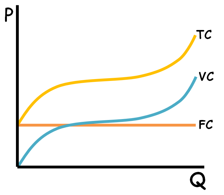
Total Costs: Variable Costs plus Fixed Costs give you Total Costs. On a graph the TC curve is the same shape as the VC. The distance between the two curves is equal to the value of the Fixed costs.
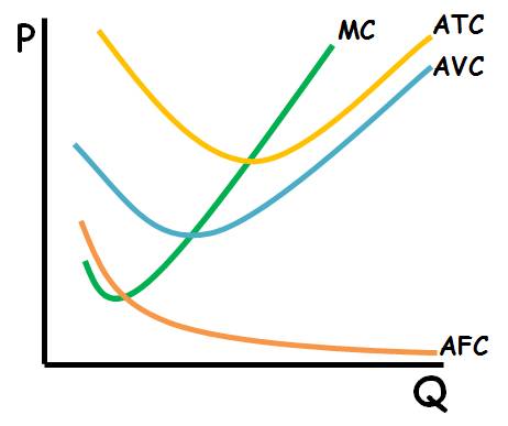
Marginal Cost: Marginal cost is the change in total cost divided by the change in quantity (MC = ∆TC/∆Q). Usually the change in quantity is just 1 so MC is the cost associated with producing just one more unit of output. The marginal cost curve intersects the ATC and AVC at their minimum points. That relationship is because as long as the cost of producing one more unit of output (MC) is less than the current average the average will fall. Also, as long as the cost of producing one more unit of output is higher than the current average, the average will rise.
The Marginal Cost curve looks like the Nike swoosh. At low quantities, the marginal cost curve is downward sloping. That is due to specialization that causes increasing marginal returns. The quantity where the marginal cost curve is at its minimum is where diminishing marginal returns sets in. Diminishing marginal returns causes marginal costs to rise at higher quantities.
Average Fixed Costs: Add up all of the fixed costs for a firm and divide by the quantity produced (AFC = FC/Q). Continually decreases. Rarely drawn because the distance between the ATC and AVC will be equal to the AFC at that quantity. Average fixed costs continually decrease as output increases.
Average Variable Costs: Add up all of the variable costs for a firm and divide by the quantity produced (AVC = VC/Q). Decreases until it intersects the MC then increases. Looks like a smirk. Firms shut down (temporarily) when price falls below the minimum point on the AVC.
Average Total Costs: Variable costs added to Fixed costs, then divided by Quantity gives you the Average Total Costs (ATC=TC/Q). It decreases until it intersects the MC then increases. Looks like a smile. The ATC tends to be a flipped average product curve. Producing the quantity where the ATC is at its minimum is productively efficient.
Shifting Cost Curves: Changing a variable cost like per unit taxes or subsidies, labor costs or raw material costs will shift the ATC, AVC, and MC upward if it is a cost increase or downward if it is a cost decrease.
Changing a fixed cost like lump sum taxes or subsidies, rent payments, or insurance payments, will only shift the ATC upward if it is a cost increase or downward if it is a cost decrease.
Long-run Costs
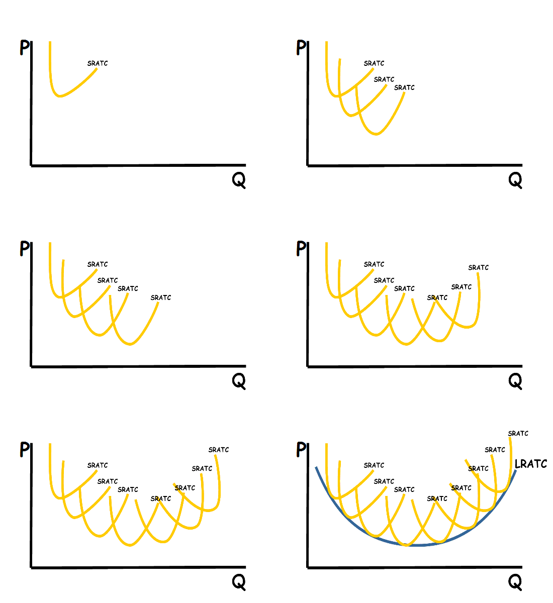
Short-run Average Total Cost (SRATC) vs Long-run Average Total Cost (LRATC): When a business first opens, it will have a short-run average total cost curve for various quantities it can produce. In the short run, only variable costs can be changed; fixed costs cannot. The firm can only change the rate of production by changing the amount of raw materials, labor, etc. it utilizes in the production process. In the long run, all costs (fixed and variable) can change. The firm can expand capacity, by purchasing more machinery or building a new factory. That change gives the firm a new short-run average total cost curve at greater quantities. As the firm continues to grow, each new capacity creates a new short-run average total cost curve at a higher quantity. Each possible SRATC gives way to a long-run average total cost curve which shows average costs for all quantities the firm can produce in the long run at every possible capacity.
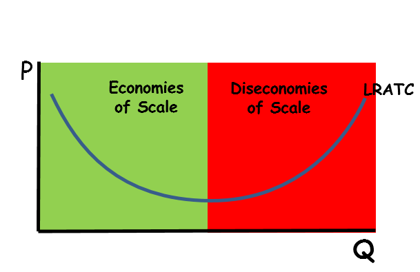
Economies of scale: When the long-run average total cost curve is downward sloping, higher quantities have a lower average cost. This occurs for many firms as they expand and get more efficient allowing them to minimize average costs. This is called economies of scale.
Many businesses will eventually reach a point where continuing to expand leads to the creation of inefficient bureaucracies, etc. which increase average costs. When this occurs, the long-run average total cost curve will be upward sloping. That is called diseconomies of scale.
Between the downward sloping and upward sloping portions of the long run average total cost curve there is often a flat portion where the firm is experiencing neither economies of scale or diseconomies of scale. This area is called constant returns to scale. Here, as the business expands production capacity, the long run average costs do not change. The smallest quantity of output where the LRATC is at it’s lowest is also called “Minimum Efficient Scale.” This is the production capacity a firm must reach in order to produce at it’s most competitive cost.
Returns to scale: One of the reasons for economies of scale is that small firms can often increase resources used by a small amount while increasing output much more. This is called increasing returns to scale. Some firms may increase output at the same rate as they increase resources. That is called constant returns to scale. Other firms may increase output at a smaller rate as they increase resources. This is called decreasing returns to scale.
The easiest way to figure out if a firm is experiencing increasing, decreasing or constant returns to scale is to double all inputs and see what happens to output. If output also doubles, the firm is experiencing constant returns to scale. If output more than doubles, it is experiencing increasing returns to scale. If output less than doubles, it is experiencing decreasing returns to scale.
Cost Curve Math
It is important to realize the shapes of all the cost curves come from a typical firm’s actual costs. The basic formulas were shown above but your next exam might make things a little trickier. Below is a chart with all costs for a fictitious firm. We will use the numbers in the chart to examine different ways to find the different costs.

Ways to find fixed cost
- Total cost for making a quantity of zero: The total cost in the example above is 20 so the fixed cost is 20
- Difference between total cost and variable cost: At the quantity of 1, the total cost is 30 and the variable cost is 10; so, the difference is 20 (30-10).
- Difference between average total cost and average variable cost times the quantity: At the quantity of 2, the average total cost is 17.5 and the average variable cost is 7.5. The difference is 10. 10 x 2 = 20, so the fixed cost is 20.
- Find average fixed cost times quantity: At the quantity of 4 the average fixed cost is 5. Since 4 x 5 = 20, the fixed cost is 20.
Ways to find marginal cost
- The change in variable cost for producing one more unit: The variable cost for a quantity of 2 is 15 and the variable cost for 3 is $25. So, the marginal cost for the 3rd unit produced is 10.
- The change in total cost for one more unit: The total cost for a quantity of 4 is 60 and the total cost for 5 is 80. So, the marginal cost for the 5th unit produced is 20.
- Multiply the average variable cost by the quantity to find variable cost. Then, find the change in the variable cost for producing one more unit. At the quantity of 4, the average variable cost is 10, so the variable cost is 40 (10 x 4 = 40). At the quantity of 5, the average variable cost is 12 so the variable cost is 60 (12 x 5 = 60). The change in variable cost for the 5th unit produced is 20 (60-40).
Ways to find variable cost
- Add all the marginal cost up to that unit: So, if you are trying to find the variable cost for the 6th unit, you would add the marginal cost for all previous units produced. The marginal cost for all 6 units is 10, 5, 10, 15, 20 and 25. Add all those up and you get a variable cost of 85.
- Total cost minus fixed cost: At a quantity of 1, the total cost is 30 and the fixed cost is 20. So, the variable cost is 10 (30-20).
- Average variable cost times quantity. At the quantity of 2, the average variable cost is 7.5. Since 2 x 7.5 = 15, the variable cost for a quantity of 2 is 15.
- Find the difference between the average total cost times the quantity and the average fixed costs times the quantity: At the quantity of 4, the average total cost is 15 and the average fixed cost is 5. Since 4 x 15 = 60 and 4 x 5 = 20, the total cost is 60 and the fixed cost is 20. The difference (the variable cost) is 40 (60-20)
- Find average variable cost times quantity: At the quantity of 5, the average variable cost is 12. Since 5 x 12 = 60, the variable cost is 60.
Ways to find the total cost
- Add the fixed cost and variable cost together: The first unit produced has a fixed cost of 20 and a variable cost of 10. So the total cost of one unit is 30 (20+10).
- Add the fixed cost and the marginal cost of each unit produced thus far: At a quantity of 2, the fixed cost is 20. The marginal cost for the first unit is 10 and the second unit is 5. Since 20+10+5=35, the total cost of 2 units is 35
- Add average variable cost times quantity and average fixed cost times quantity together: At the quantity of 5, the average variable cost is 12 and the average fixed cost is 4. Since 5 x 12 = 60 and 5 x 4 = 20, the total cost for 5 units is 80 (60+20).
- Find average total cost times quantity: At 6 units, the average total cost is 17.5. Since 6 x 17.5 = 105, the average total cost for 6 units is 105.
Ways to find average variable cost
- Find variable cost (using any method above) and divide by quantity: At the quantity of 2, the variable cost is 15. Since 15/2 = 7.5, the average variable cost for 2 units is 7.5.
- Difference between average total cost and average fixed cost: At the quantity of 3, the average total cost is 15 and the average fixed cost is 6.67. Since 15 – 6.67 = 8.33.
Ways to find average total cost
- Find total cost (using any method above) and divide by quantity: At the quantity of 3, the total cost is 45. Since 45/3 = 15, the average total cost for 3 units is 15.
- Add average variable cost and average fixed cost: At the quantity of 4, the average variable cost is 10 and the average fixed 5. Since 10 + 5 = 15, the average total cost for 4 units is 15.
Ways to find average fixed cost
- Find fixed cost (using any method above) and divide by quantity: At the quantity of 5, the fixed cost is 20. Since 20/5 = 4 the average fixed cost for 5 units is 4.
- Difference between average total cost and average variable cost: At the quantity of 6, the average total cost is 17.5 and the average variable cost is 14.17. Since 17.5 – 14.17 = 3.33, the average fixed cost for 6 units is 3.33.
Multiple Choice Connections:
2012 Released AP Microeconomics Exam Questions: 7, 22, 25, 37, 50
Up Next:
Review Game: Cost Curve Calculations Practice, Shading Practice, and Prices, Points, and Quantities
Content Review Page: 4 Product Market Structures
Other recommended resources: Jodi Econ Girl (Short Run Cost Curves), Long Run Cost (ACDC Leadership)
